
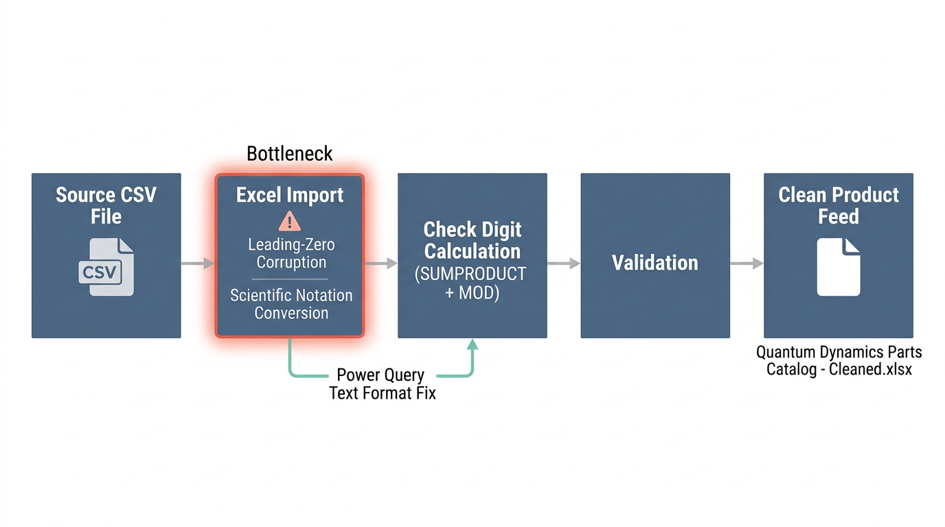
The GS1 check digit uses MOD 10 with alternating ×3 and ×1 weights. You can calculate it in Excel with SUMPRODUCT, MID, and MOD. But here's the catch: if your GTINs are stored as numbers, Excel has already corrupted them before any formula runs. Fix the storage type first.
The silent corruption problem
Excel does two things to GTINs that destroy your data before you even touch a formula.
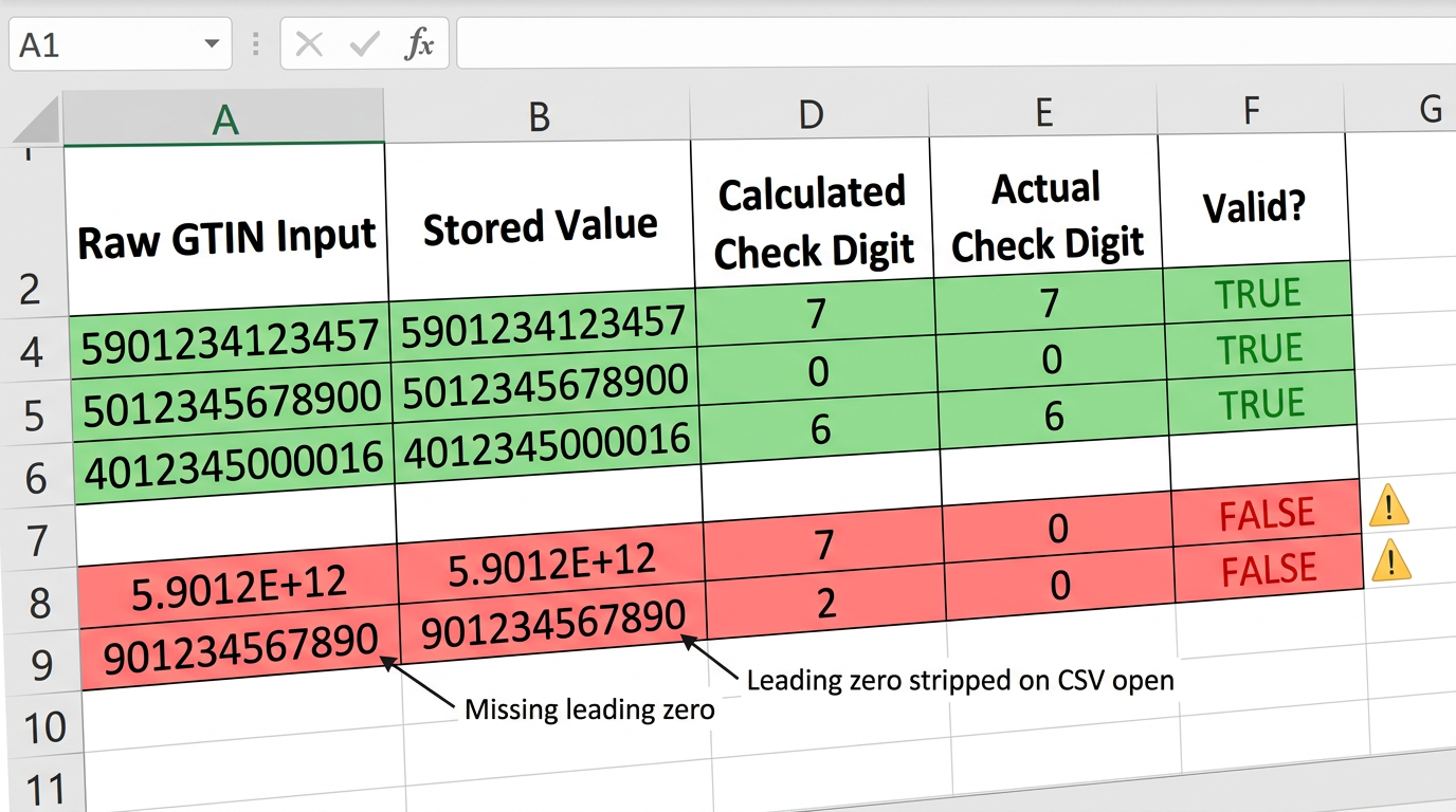
First, it strips leading zeros. A GTIN like 0614141007349 becomes 614141007349 the moment you paste it into a default cell. Wrong length. Wrong check digit lookup. Second, Excel converts any number over 15 significant digits to scientific notation. Your GTIN-14 shows up as 1.06141E+13. Try running MID() on that.
This isn't a bug. It's how Excel handles numbers. The fix is simple: tell Excel it's text before the data arrives.
Pasted as numbers
- 0614141007349 → 614141007349 (leading zero gone)
- 10614141007346 → 1.06141E+13 (scientific notation)
- 5901234123457 → 5901234123457 (looks fine, actually fine)
- 00012345678905 → 12345678905 (two zeros gone)
Stored as Text
- 0614141007349 → 0614141007349 ✓
- 10614141007346 → 10614141007346 ✓
- 5901234123457 → 5901234123457 ✓
- 00012345678905 → 00012345678905 ✓
Two ways to get this right. Format your destination column as Text before pasting. Or use Power Query's From Text/CSV wizard and set the GTIN column type to Text during import. Do this first. Every formula below assumes your GTINs are stored correctly.
How the check digit algorithm works
GS1 uses the same algorithm for GTIN-8, GTIN-12, GTIN-13, and GTIN-14. Take all digits except the last one. Multiply each by alternating weights of 1 and 3, starting from the rightmost digit. Sum the products. The check digit is whatever you need to add to make the sum divisible by 10.
The formula: (10 − (sum MOD 10)) MOD 10
Here's 590123412345 worked out digit by digit:
| Position | Digit | Weight | Product |
|---|---|---|---|
| 1 | 5 | 1 | 5 |
| 2 | 9 | 3 | 27 |
| 3 | 0 | 1 | 0 |
| 4 | 1 | 3 | 3 |
| 5 | 2 | 1 | 2 |
| 6 | 3 | 3 | 9 |
| 7 | 4 | 1 | 4 |
| 8 | 1 | 3 | 3 |
| 9 | 2 | 1 | 2 |
| 10 | 3 | 3 | 9 |
| 11 | 4 | 1 | 4 |
| 12 | 5 | 3 | 15 |
| Sum | 83 |
(10 − (83 MOD 10)) MOD 10 = (10 − 3) MOD 10 = 7
Full barcode: 5901234123457. You can verify this against the GS1 check digit calculator. Or try it in our GTIN validator, which checks the digit and flags common format problems in one step.
The Excel formula for GTIN-13
Building this in Excel means extracting each digit, applying the weight, and summing. SUMPRODUCT does the heavy lifting.
Format column A as Text before pasting. Your 12-digit input goes in A2.
MID(A2,1,1) gets the first digit. MID(A2,2,1) gets the second. You'll need all 12.
Multiply positions 1,3,5,7,9,11 by 1. Multiply positions 2,4,6,8,10,12 by 3. SUMPRODUCT lets you do this in one shot.
Take the sum MOD 10. Subtract from 10. Take that result MOD 10. Done.
Generator formula (input is 12 digits without check digit, cell A2):
=MOD(10-MOD(SUMPRODUCT(--MID(A2,{1,2,3,4,5,6,7,8,9,10,11,12},1),{1,3,1,3,1,3,1,3,1,3,1,3}),10),10)
Validation formula (input is full 13-digit GTIN, cell A2):
=MOD(10-MOD(SUMPRODUCT(--MID(A2,{1,2,3,4,5,6,7,8,9,10,11,12},1),{1,3,1,3,1,3,1,3,1,3,1,3}),10),10)=VALUE(RIGHT(A2,1))
This returns TRUE if the check digit matches, FALSE if it doesn't.
Adapting for GTIN-8, GTIN-12, and GTIN-14
GS1 always pads shorter GTINs to 14 digits with leading zeros before applying weights. The positional logic stays the same. You just need different array lengths.
| Type | Total digits | Input digits | Weight array |
|---|---|---|---|
| GTIN-8 | 8 | 7 | |
| GTIN-12 | 12 | 11 | |
| GTIN-13 | 13 | 12 | |
| GTIN-14 | 14 | 13 |
Notice the pattern. GTIN-14 starts with weight 3. GTIN-13 starts with weight 1. This is because padding to 14 digits shifts everything.
Full GTIN already in the cell: use the validation formula for that length. Digits without check digit: use the generator formula, match array to input length. Mixed lengths in the same column: pad inputs to 13 digits with TEXT(A2,REPT("0",13)), then use GTIN-14 weights. Cell shows E+12 or E+13: stop. Fix the storage type. Then run formulas.
Bulk validation in two minutes
You've got 500 GTINs from a supplier. Put the validation formula in column C, drag it down, then apply conditional formatting to highlight failures.
Supplier feed from Volterra Supply Co.
| SKU | Supplier GTIN | Valid? |
|---|---|---|
| NRG-4401 | 5901234123457 | TRUE |
| NRG-4402 | 4006381333931 | TRUE |
| NRG-4403 | 5901234123458 | FALSE |
| NRG-4404 | 0614141007349 | TRUE |
| NRG-4405 | 7350053850019 | TRUE |
| NRG-4406 | 4006381333932 | FALSE |
Formula in C2: =MOD(10-MOD(SUMPRODUCT(--MID(B2,{1,2,3,4,5,6,7,8,9,10,11,12},1),{1,3,1,3,1,3,1,3,1,3,1,3}),10),10)=VALUE(RIGHT(B2,1))
Rows 3 and 6 fail. The check digits are off by one.
For conditional formatting: select your GTIN column, create a rule that formats cells where the adjacent validation column equals FALSE. Red fill works. Now every bad barcode lights up.
When you find failures, go back to the supplier with the row numbers and the calculated versus actual check digit. They need to fix their source data. Validating downstream won't help if the upstream file keeps shipping bad barcodes. If you're unsure whether to use GTIN-13, EAN, or UPC in your feed, see GTIN vs EAN vs UPC for the definitive breakdown.